Colligative properties refer to the physical changes that result from adding solute to a solvent. Colligative properties depend on the number of solute particles and the amount of solvent. Precisely, they depend on the ratio of the number of solute particles to the number of solvent particles in a solution. The number ratio can be expressed in the solution’s concentration units, such as molarity, molality, and normality. ^[1-4]

Colligative properties do not depend on the type of solute particles, even though they do depend on the type of solvent. An assumption for colligative properties is that the solution must be ideal; their thermodynamic properties must be analogous to an ideal gas.

Types of Colligative Properties

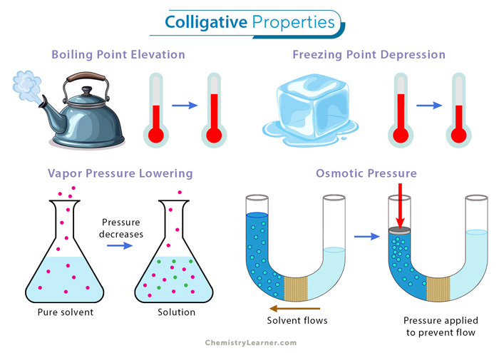
The four colligative properties occurring in a solution are: ^[1-4]

• Vapor Pressure Depression
• Boiling Point Elevation 
• Freezing Point Depression
• Osmotic Pressure

Example

The demonstration of colligative properties in solutions becomes apparent when considering the following instances. For example, upon introducing a small amount of salt to a glass of water, the solution’s freezing point significantly decreases compared to the water’s freezing point. Similarly, the boiling point of the solution rises, resulting in reduced vapor pressure. Moreover, alterations in the solution’s osmotic pressure also become evident.

Let us study in detail the abovementioned colligative properties.

1. Vapor Pressure Depression

Every pure liquid exhibits a unique vapor pressure when in equilibrium with its liquid phase. The partial pressure associated with this equilibrium is intricately linked to temperature. In the case of solutions, their vapor pressure is notably lower than that of the pure solvent. The extent of this reduction depends upon the proportion of solute particles present, assuming the solute itself does not possess a substantial vapor pressure. Solute substances lacking significant vapor pressure are termed non-volatile. This phenomenon is recognized as vapor pressure depression or lowering.

The computation of the actual vapor pressure of a solution involves the following formula:

P_soln = χ_solv * P^o_solv

Here, P_soln signifies the vapor pressure of the solution,​ χ_solv represents the mole fraction of solvent particles, and P^o_solv​​ stands for the vapor pressure of the pure solvent at the given temperature. This equation is commonly referred to as Raoult’s law. The rationale behind vapor pressure depression is based on the assumption that solute particles occupy positions on the surface, displacing solvent particles. Consequently, the evaporation of solvent particles is hindered due to this displacement by solute particles.

2. Boiling Point Elevation

Due to the presence of a non-volatile solute in a solution, the vapor pressure of the solution becomes lower than that of the pure solvent. Consequently, achieving a vapor pressure of 1 atm or 760 torr necessitates a higher temperature for the solution than the pure solvent. This temperature at which the liquid’s vapor pressure reaches 1 atm is the standard boiling point. Thus, the solution’s standard boiling point surpasses the pure solvent, a phenomenon referred to as boiling point elevation.

The change in boiling point, denoted as ΔT_b, can be easily computed using the formula:

ΔT_b = m * K_b

In this equation, m represents the molality of the solution (mol/kg), and K_b is the boiling point elevation constant, an inherent trait of the solvent. It is crucial to note that the initial calculation yields the change in boiling point temperature, not the new temperature. After determining the change in boiling point temperature, it must be added to the boiling point of the pure solvent. This step is essential since boiling points consistently experience elevation, ultimately yielding the new boiling point of the solution.

3. Freezing Point Depression

We have seen that the solution’s boiling point exceeds that of the pure solvent. An inverse effect is observed concerning the freezing point. The freezing point of the solution reduces below that of the pure solvent. This phenomenon can be visualized by considering how solute particles disrupt the cohesion of solvent particles during the formation of a solid, necessitating a lower temperature to induce solidification. Known as freezing point depression, this occurrence is responsible for the lowered freezing point.

The formula employed to compute the change in freezing point (ΔT_b) for a solution is analogous to the one used for the elevation of the boiling point:

ΔT_f = m * K_f

Here, m denotes the molality of the solution (mol/kg), and K_f is referred to as the freezing point depression constant, a unique attribute of the solvent.

It is crucial to note that the formula above calculates the shift in freezing point, not the new freezing point itself. The value derived from the calculation must be subtracted from the standard freezing point of the solvent, as freezing points inherently decrease.

Application of Freezing Point Depression in Real Life

Freezing point depression is a significant colligative property applicable to our daily lives. Numerous antifreeze solutions utilized in vehicle radiators are engineered to possess diminished freezing points, enabling automobile engines to function in subfreezing conditions. Additionally, we utilize the principle of freezing point depression when spreading different substances on icy surfaces to expedite thawing during winter for safety purposes. These substances create solutions with lowered freezing points, causing any existing ice to melt into liquid and drain away, ultimately leaving a safer pavement surface.

4. Osmotic Pressure

A semipermeable membrane is a physical object that allows certain substances to pass through and prevents others. Placing a semipermeable membrane between a solution and solvent reveals an intriguing phenomenon. Solvent molecules permeate through the membrane into the solution, causing an increase in the solution’s volume. The semipermeable nature of the membrane allows passage solely for solvent molecules while effectively blocking larger molecules like the solute. This spontaneous movement of solvent molecules through the semipermeable membrane, from a pure solvent to a solution or from a dilute to a concentrated solution, is termed osmosis.

The movement of solvent molecules across the semipermeable membrane can be obstructed by applying additional pressure from the solution side. This defensive pressure against the solvent flow is the solution’s osmotic pressure.

Osmotic pressure is a colligative property, deriving its behavior from the number of solutes present rather than their specific characteristics. Experimental evidence validates that the osmotic pressure (Π) is directly proportional to molarity (M), temperature (T), and vant Hoff factor (i). Mathematically, this relationship can be expressed as 

Π = i * M * R * T

where the gas constant is denoted as R.

This equation can also be represented as 

Π = (n₂/V) RT

where V signifies the volume of the solution in liters, and n₂ represents the number of moles of the solute.

If the mass of the solute is denoted as m₂ and its molar mass as M₂, then n₂ can be calculated as

n₂ = m₂/M₂.

It leads to the following formulation: 

Π = m₂RT/M₂V,

Therefore, given the values of osmotic pressure (Π), solute mass (m₂), temperature (T), and volume (V), it becomes feasible to calculate the molar mass of the solute through this equation.

Example Problems

Problem 1. Calculate the vapor pressure of a solution prepared by dissolving 25 g of glucose in 200 g of water at 27 °C. The vapor pressure of pure water at 27 °C is 26.74 torr. (Molecular masses of glucose and water are 180 g/mol and 18 g/mol, respectively) 

Solution

Given m₂ = 25 g, m₁ = 200 g, T = 27 °C = 27 + 273 = 300 K, P^o_solv = 26.74 torr

We use the following formula:

P_soln = χ_solv × P^o_solv

To calculate the molar fraction of the solvent, we use the following formula:

χ_solv = n₁/(n₁ + n₂)

Let us calculate the number of moles of glucose and water present in the solution.

n₁ = 200 g/18 g/mol = 11.1 mol

n₂ = 25 g/180 g/mol = 0.139 mol

We have,

χ_solv = 11.1 mol/(11.1 mol + 0.139 mol) = 0.988 

And,

P_soln = 0.988 × 26.74 torr = 26.41 torr

Therefore, water’s vapor pressure is reduced from 26.74 torr to 26.41 torr.

Problem 2. A sample of 1 g of a non-volatile organic compound is dissolved in 50 g benzene. The BP of the solution is 81.06 °C. BP of pure benzene is 80.08 °C. What is the molar mass of the solute? (Boiling point elevation constant for benzene is 2.53 °C kg mol^-1)

Solution

Given m₂ = 1 g, m₁ = 50 g, T_{B, soln} = 81.06 °C, T^o_{B, solv} = 80.08 °C, and k_B = 2.53 °C kg mol^-1

We use the following formula:

ΔT_B = m * K_B

=> 81.06 °C – 80.08 °C = m * 2.53 °C kg mol^-1

=> m = 0.387 mol kg^-1

The number of moles of the solute is

n = m * m₁ = 0.387 mol kg^-1 * 50 g x 10^-3 kg/g = 0.019 mol

The molar mass of the solute is

M = m₂/n = 1 g / 0.019 mol = 51.6 g/mol